Classification

Classifiers

After recording, processing, and extracting features from a window of EMG data, it is passed to a machine learning algorithm for classification. These control systems have evolved in the prosthetics community for continuously classifying muscular contractions for enabling prosthesis control. Therefore, they are primarily limited to recognizing static contractions (e.g., hand open/close and wrist flexion/extension) as they have no temporal awareness. Currently, this is the form of recognition supported by LibEMG and is an initial step to explore EMG as an interaction opportunity for general-purpose use. This section highlights the machine-learning strategies that are part of LibEMG’s pipeline. Additionally, a number of post-processing methods (i.e., techniques to improve performance after classification) are explored.

Statistical Models

The statistical classifiers (i.e., traditional machine learning methods) implemented leverage the sklearn package. For most cases, the “base” classifiers use the default options, meaning that the pre-defined models are not necessarily optimal. However, the parameters attribute can be used when initializing the classifiers to pass in additional sklearn parameters in a dictionary. For example, looking at the RandomForestClassifier docs on sklearn:

Random Forest

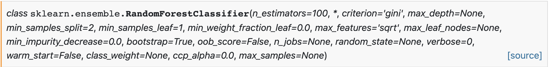
A classifier with any of those parameters using the parameters attribute. For example:

parameters = {
    'n_estimators': 99,
    'max_depth': 20,
    'random_state': 5,
    'max_leaf_nodes': 10
}
classifier = EMGClassifier('RF', data_set, parameters=parameters)

Please reference the sklearn docs for parameter options for each classifier.

Additionally, custom classifiers can be created. Any custom classifier should be modeled after the sklearn classifiers and must have the fit, predict, and predict_proba functions to work correctly.

from sklearn.ensemble import RandomForestClassifier
from libemg.classification import EMGClassifier

rf_custom_classifier = RandomForestClassifier(max_depth=5, random_state=0)
classifier = EMGClassifier()
classifier.fit(rf_custom_classifier, data_set)

Linear Discriminant Analysis (LDA)

A linear classifier that uses common covariances for all classes and assumes a normal distribution.

classifier = EMGClassifier()
classifier.fit('LDA', data_set)

Check out the LDA docs here.

K-Nearest Neighbour (KNN)

Discriminates between inputs using the K closest samples in feature space. The implemented version in the library defaults to k = 5. A commonly used classifier for EMG-based recognition.

params = {'n_neighbors': 5} # Optional
classifier = EMGClassifier()
classifier.fit('KNN', data_set, parameters=params)

Check out the KNN docs here.

Support Vector Machines (SVM)

A hyperplane that maximizes the distance between classes is used as the boundary for recognition. A commonly used classifier for EMG-based recognition.

classifier = EMGClassifier()
classifier.fit('SVM', data_set)

Check out the SVM docs here.

Artificial Neural Networks (MLP)

A deep learning technique that uses human-like “neurons” to model data to help discriminate between inputs. Especially for this model, we highly recommend you create your own.

classifier = EMGClassifier()
classifier.fit('MLP', data_set)

Check out the MLP docs here.

Random Forest (RF)

Uses a combination of decision trees to discriminate between inputs.

classifier = EMGClassifier()
classifier.fit('RF', data_set)

Check out the RF docs here.

Quadratic Discriminant Analysis (QDA)

A quadratic classifier that uses class-specific covariances and assumes normally distributed classes.

classifier = EMGClassifier()
classifier.fit('QDA', data_set)

Check out the QDA docs here.

Gaussian Naive Bayes (NB)

Assumes independence of all input features and normally distributed classes.

classifier = EMGClassifier()
classifier.fit('NB', data_set)

Check out the NB docs here.

Deep Learning (Pytorch)

Another available option is to use pytorch models (i.e., a library for deep learning) to train the classifier, although this involves making some custom code for preparing the dataset and the deep learning model. For a guide on how to use deep learning models, consult the deep learning example.

Post-Processing

Rejection

Classifier outputs are overridden to a default or inactive state when the output decision is uncertain. This concept stems from the notion that it is often better (less costly) to incorrectly do nothing than it is to erroneously activate an output.

Confidence ^[1]: Rejects based on a predefined confidence threshold (between 0-1). If predicted probability is less than the confidence threshold, the decision is rejected. Figure 1 exemplifies rejection using an SVM classifier with a threshold of 0.8.

# Add rejection with 90% confidence threshold
classifier.add_rejection(threshold=0.9)

Majority Voting ^[2,3]

Overrides the current output with the label corresponding to the class that occurred most frequently over the past \(N\) decisions. As a form of simple low-pass filter, this introduces a delay into the system but reduces the likelihood of spurious false activations. Figure 1 exemplifies applying a majority vote of 5 samples to a decision stream.

# Add majority vote on 10 samples
classifier.add_majority_vote(num_samples=10)

Velocity Control ^[4]

Outputs an associated velocity with each prediction that estimates the level of muscular contractions (normalized by the particular class). This means that within the same contraction, users can contract harder or lighter to control the velocity of a device. Note that ramp contractions should be accumulated during the training phase.

# Add velocity control
classifier.add_velocity(train_windows, train_labels)

Figure 1 shows the decision stream (i.e., the predictions over time) of a classifier with no post-processing, rejection, and majority voting. In this example, the shaded regions show the ground truth label, whereas the colour of each point represents the predicted label. All black points indicate predictions that have been rejected.

alt text

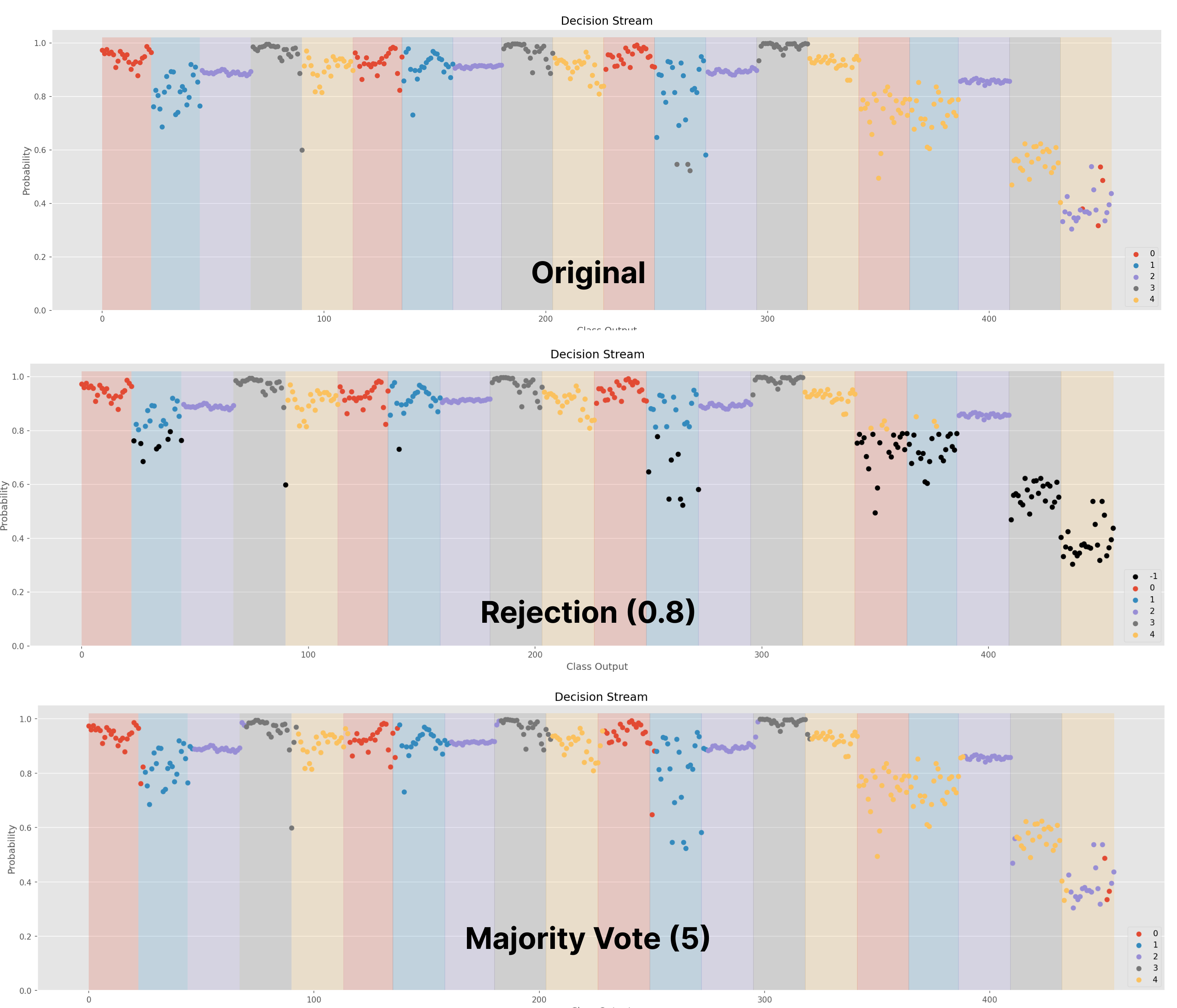
Figure 1: Decision Stream of No Post-Processing, Rejection, and Majority Voting. This can be created using the .visualize() method call.

References

[1] E. J. Scheme, B. S. Hudgins and K. B. Englehart, “Confidence-Based Rejection for Improved Pattern Recognition Myoelectric Control,” in IEEE Transactions on Biomedical Engineering, vol. 60, no. 6, pp. 1563-1570, June 2013, doi: 10.1109/TBME.2013.2238939.

[2] Scheme E, Englehart K. Training Strategies for Mitigating the Effect of Proportional Control on Classification in Pattern Recognition Based Myoelectric Control. J Prosthet Orthot. 2013 Apr 1;25(2):76-83. doi: 10.1097/JPO.0b013e318289950b. PMID: 23894224; PMCID: PMC3719876.

[3] Wahid MF, Tafreshi R, Langari R. A Multi-Window Majority Voting Strategy to Improve Hand Gesture Recognition Accuracies Using Electromyography Signal. IEEE Trans Neural Syst Rehabil Eng. 2020 Feb;28(2):427-436. doi: 10.1109/TNSRE.2019.2961706. Epub 2019 Dec 23. PMID: 31870989.

[4] E. Scheme, B. Lock, L. Hargrove, W. Hill, U. Kuruganti and K. Englehart, “Motion Normalized Proportional Control for Improved Pattern Recognition-Based Myoelectric Control,” in IEEE Transactions on Neural Systems and Rehabilitation Engineering, vol. 22, no. 1, pp. 149-157, Jan. 2014, doi: 10.1109/TNSRE.2013.2247421.

[Sklearn] Fabian Pedregosa, Gaël Varoquaux, Alexandre Gramfort, Vincent Michel, Bertrand Thirion, Olivier Grisel, Mathieu Blondel, Peter Prettenhofer, Ron Weiss, Vincent Dubourg, Jake Vanderplas, Alexandre Passos, David Cournapeau, Matthieu Brucher, Matthieu Perrot, and Édouard Duchesnay. 2011. Scikit-learn: Machine Learning in Python. J. Mach. Learn. Res. 12, null (2/1/2011), 2825–2830.